Ensemble Clustered Inference on 2D Data

In this example, we present how to perform inference on simulated 2D data. This setting is particularly challenging since the number of features (pixels in 2D) is much larger than the number of samples. We first illustrate the limitations of the Desparsified Lasso method in this setting and then present two methods that leverage the data’s spatial structure to build clusters and perform the inference at the cluster level. We first show how to use clustered inference with DL (hidimstat.CluDL). We then show how to use clustered inference with Ensembled CluDL (hidimstat.EnCluDL).

Generating the data

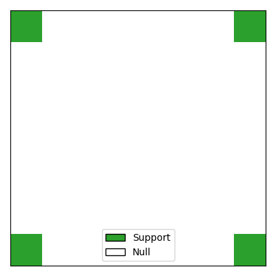
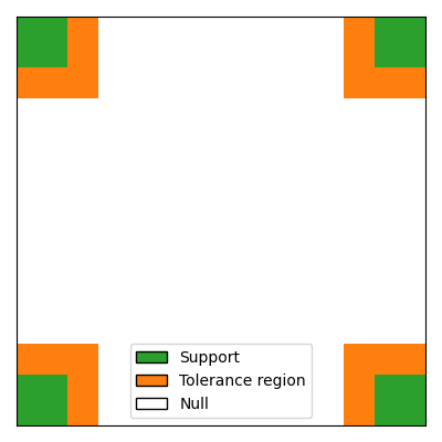
We begin by simulating 2D data where the support (i.e., the predictive features) consists of four regions of neighboring pixels located in each corner of the 2D image. The target variable \(y\) is a continuous variable generated from a linear model. To make the problem more challenging, the pixels are spatially correlated using a Gaussian filter.

import matplotlib.pyplot as plt
import seaborn as sns
from matplotlib.colors import ListedColormap
from matplotlib.patches import Patch

from hidimstat._utils.scenario import multivariate_simulation_spatial

n_samples = 100
shape = (40, 40)
n_features = shape[1] * shape[0]
roi_size = 5  # size of the edge of the four predictive regions
signal_noise_ratio = 16.0  # noise standard deviation
smooth_X = 1.0  # level of spatial smoothing introduced by the Gaussian filter

# generating the data
X_init, y, beta, epsilon = multivariate_simulation_spatial(
    n_samples, shape, roi_size, signal_noise_ratio, smooth_X, seed=0
)
print(f"Number of samples: {X_init.shape[0]}, Number of features: {n_features}")


# visualize the data
cmap = ListedColormap(["white", "tab:green"])  # 0 -> blue (null), 1 -> green (support)
fig, ax = plt.subplots(figsize=(4, 4), subplot_kw={"xticks": [], "yticks": []})
ax.imshow(
    beta.reshape(shape),
    cmap=cmap,
    vmin=0,
    vmax=1,
)

# Legend: green = support, blue = null
legend_handles = [
    Patch(facecolor="tab:green", edgecolor="k", label="Support"),
    Patch(facecolor="white", edgecolor="k", label="Null"),
]
ax.legend(handles=legend_handles, loc="lower center")
plt.tight_layout()

Number of samples: 100, Number of features: 1600

Inference with Desparsified Lasso

First, we perform inference using the Desparsified Lasso method, treating the data as a standard high-dimensional regression problem without considering its spatial structure. The aim of the inference step is to recover the support while controlling the Family-Wise Error Rate (FWER) at a targeted level of 0.1. To achieve this, we use the Bonferroni correction, applying a factor equal to the number of features. For more details about the Desparsified Lasso method, see Javanmard and Montanari[1], Zhang and Zhang[2] and van de Geer et al.[3].

import numpy as np
from sklearn.linear_model import LassoCV

from hidimstat import DesparsifiedLasso

fwer_target = 0.1
n_jobs = 5  # number of workers for parallel computing

# compute desparsified lasso
estimator = LassoCV(max_iter=1000, tol=0.0001, eps=0.01, fit_intercept=False)
dl = DesparsifiedLasso(estimator=estimator, n_jobs=n_jobs, random_state=0)
dl.fit_importance(X_init, y)

# compute estimated support (first method)
selected_dl = dl.fwer_selection(fwer=fwer_target, n_tests=n_features)

tp_mask = ((selected_dl.astype(int) == 1) & (beta == 1)).astype(bool)
fp_mask = ((selected_dl.astype(int) == 1) & (beta == 0)).astype(bool)
fn_mask = ((selected_dl.astype(int) == 0) & (beta == 1)).astype(bool)
mask_dl = np.zeros(shape)
mask_dl[tp_mask.reshape(shape)] = 1
mask_dl[fp_mask.reshape(shape)] = -2
mask_dl[fn_mask.reshape(shape)] = -1

/home/circleci/project/.venv/lib/python3.13/site-packages/sklearn/linear_model/_coordinate_descent.py:695: ConvergenceWarning: Objective did not converge. You might want to increase the number of iterations, check the scale of the features or consider increasing regularisation. Duality gap: 8.696e-01, tolerance: 8.364e-01
  model = cd_fast.enet_coordinate_descent(

We visualize the support estimated by the Desparsified Lasso method.

_, ax = plt.subplots(figsize=(4, 4), subplot_kw={"xticks": [], "yticks": []})
cmap = ListedColormap(["tab:red", "tab:purple", "white", "tab:green"])
ax.imshow(mask_dl, cmap=cmap, vmin=-2, vmax=1)
legend_handles = [
    Patch(facecolor="tab:green", edgecolor="k", label="True Positive"),
    Patch(facecolor="tab:red", edgecolor="k", label="False Positive"),
    Patch(facecolor="tab:purple", edgecolor="k", label="False Negative"),
]
ax.legend(handles=legend_handles, loc="lower center")
plt.tight_layout()

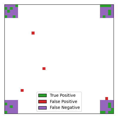
It can be seen that: 1. the Desparsified Lasso method is not powerful enough to recover the support, it only selects scattered pixels as true positives without identifying the regions. 2. the number of false positives is quite high, and sometimes false positives are located far from the true support.

Clustered inference with CluDL

To improve the power of the inference, we can leverage the spatial structure of the data. The idea is to group correlated pixels into clusters, using an additional spatial constraint (pixels are iteratively merged with neighboring pixels). This approach leads to a dimension reduction while preserving the data’s spatial structure. To control the FWER at the targeted level of 0.1, we perform Bonferroni correction, but here the correction factor is equal to the number of clusters instead of the number of features. For more details about CluDL, see Chevalier et al.[4].

from sklearn.base import clone
from sklearn.cluster import FeatureAgglomeration
from sklearn.feature_extraction import image

from hidimstat import CluDL

# Clustering step
n_clusters = 200
connectivity = image.grid_to_graph(n_x=shape[0], n_y=shape[1])
clustering = FeatureAgglomeration(
    n_clusters=n_clusters, connectivity=connectivity, linkage="ward"
)

dl_2 = DesparsifiedLasso(estimator=clone(estimator), n_jobs=n_jobs)
clu_dl = CluDL(desparsified_lasso=dl_2, clustering=clustering, random_state=0)
clu_dl.fit_importance(X_init, y)

selected_cdl = clu_dl.fwer_selection(fwer=fwer_target, n_tests=n_clusters)

Visualizing the support estimated by CluDL

tp_mask = ((selected_cdl.astype(int) == 1) & (beta == 1)).astype(bool)
fp_mask = ((selected_cdl.astype(int) == 1) & (beta == 0)).astype(bool)
fn_mask = ((selected_cdl.astype(int) == 0) & (beta == 1)).astype(bool)
mask_cludl = np.zeros(shape)
mask_cludl[tp_mask.reshape(shape)] = 1
mask_cludl[fp_mask.reshape(shape)] = -2
mask_cludl[fn_mask.reshape(shape)] = -1

_, ax = plt.subplots(figsize=(4, 4), subplot_kw={"xticks": [], "yticks": []})
cmap = ListedColormap(["tab:red", "tab:purple", "white", "tab:green"])
ax.imshow(mask_cludl, cmap=cmap, vmin=-2, vmax=1)
legend_handles = [
    Patch(facecolor="tab:green", edgecolor="k", label="True Positive"),
    Patch(facecolor="tab:red", edgecolor="k", label="False Positive"),
    Patch(facecolor="tab:purple", edgecolor="k", label="False Negative"),
]
ax.legend(handles=legend_handles, loc="lower center")
plt.tight_layout()

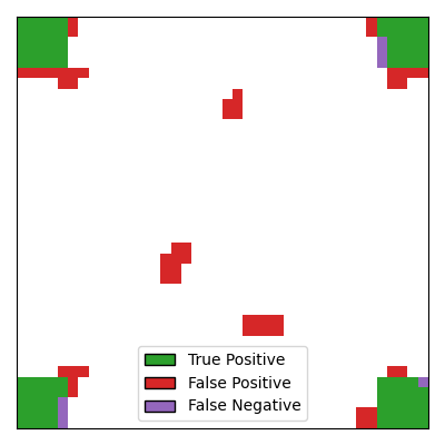
With CluDL, the support recovery is more powerful, with large regions of the true support being correctly identified. However, some false positives remain. In this case, these false positives consist of small clusters that can be either contiguous to the true support or located far from it.

Inference with Ensembled CluDL

Finally, we perform inference using an ensembled version of CluDL called EnCluDL. The idea is to run several CluDL algorithms with different clustering choices. By repeating the clustering step on different bootstrap samples of the data, this approach derandomizes the clustering choice and makes it more robust to small variations in the data. It can be efficiently parallelized since the different CluDL runs are independent and thus embarrassingly parallel. Similar to CluDL, we perform Bonferroni correction with a factor equal to the number of clusters on the p-values obtained by aggregating the different CluDL runs. For more details about EnCluDL, see Chevalier et al.[4].

from hidimstat.ensemble_clustered_inference import EnCluDL

enclu_dl = EnCluDL(
    desparsified_lasso=DesparsifiedLasso(estimator=clone(estimator), n_jobs=1),
    clustering=clustering,
    n_bootstraps=20,
    random_state=0,
    n_jobs=n_jobs,
    cluster_boostrap_size=0.5,
)
enclu_dl.fit_importance(X_init, y)

selected_ecdl = enclu_dl.fwer_selection(fwer=fwer_target, n_tests=n_clusters)

Fitting clustered inferences:   0%|          | 0/20 [00:00<?, ?it/s]
Fitting clustered inferences:  50%|█████     | 10/20 [00:00<00:00, 20.30it/s]
Fitting clustered inferences:  75%|███████▌  | 15/20 [00:00<00:00, 14.18it/s]
Fitting clustered inferences: 100%|██████████| 20/20 [00:01<00:00, 11.42it/s]
Fitting clustered inferences: 100%|██████████| 20/20 [00:01<00:00, 12.70it/s]

Computing importances:   0%|          | 0/20 [00:00<?, ?it/s]
Computing importances: 100%|██████████| 20/20 [00:00<00:00, 335.46it/s]

Visualizing the support estimated by EnCluDL

tp_mask = ((selected_ecdl.astype(int) == 1) & (beta == 1)).astype(bool)
fp_mask = ((selected_ecdl.astype(int) == 1) & (beta == 0)).astype(bool)
fn_mask = ((selected_ecdl.astype(int) == 0) & (beta == 1)).astype(bool)
mask_encludl = np.zeros(shape)
mask_encludl[tp_mask.reshape(shape)] = 1
mask_encludl[fp_mask.reshape(shape)] = -2
mask_encludl[fn_mask.reshape(shape)] = -1


_, ax = plt.subplots(figsize=(4, 4), subplot_kw={"xticks": [], "yticks": []})
cmap = ListedColormap(["tab:red", "tab:purple", "white", "tab:green"])
ax.imshow(mask_encludl, cmap=cmap, vmin=-2, vmax=1)
legend_handles = [
    Patch(facecolor="tab:green", edgecolor="k", label="True Positive"),
    Patch(facecolor="tab:red", edgecolor="k", label="False Positive"),
    Patch(facecolor="tab:purple", edgecolor="k", label="False Negative"),
]
ax.legend(handles=legend_handles, loc="lower center")
plt.tight_layout()

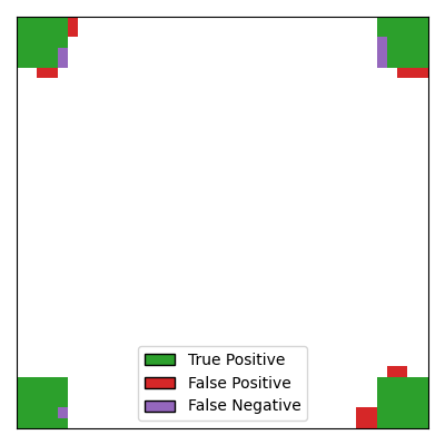
Compared to CluDL, EnCluDL further improves the inference, primarily by reducing the number of false positives located far from the true support. An intuitive explanation for this improvement is that while false discoveries far from the true support may occur randomly in a single clustering, they are less likely to occur repeatedly in overlapping clusters obtained from different bootstrap samples of the data.

Support recovery with spatial tolerance

For spatially structured data, false discoveries that are close to the true support, or even part of clusters that intersect the true support, are likely to change less the interpretation of the results than false discoveries located far from the support. Therefore, it can be relevant to consider a spatially relaxed support recovery, The idea is to penalize less those false discoveries that are close to the true support. To achieve this, we introduce an extended support that includes the true support and a tolerance region around it.

spatial_tolerance = 3
roi_size_extended = roi_size + spatial_tolerance
beta_extended = beta.copy().reshape(shape)
beta_extended[0:roi_size_extended, 0:roi_size_extended] += 1
beta_extended[-roi_size_extended:, -roi_size_extended:] += 1
beta_extended[0:roi_size_extended, -roi_size_extended:] += 1
beta_extended[-roi_size_extended:, 0:roi_size_extended] += 1

# visualize the extended support
cmap = ListedColormap(["white", "tab:orange", "tab:green"])
fig, ax = plt.subplots(figsize=(4, 4), subplot_kw={"xticks": [], "yticks": []})
ax.imshow(beta_extended.reshape(shape), cmap=cmap, vmin=0, vmax=2)
# Legend: green = support, yellow = tolerance region, white = null
legend_handles = [
    Patch(facecolor="tab:green", edgecolor="k", label="Support"),
    Patch(facecolor="tab:orange", edgecolor="k", label="Tolerance region"),
    Patch(facecolor="white", edgecolor="k", label="Null"),
]
ax.legend(handles=legend_handles, loc="lower center")
plt.tight_layout()

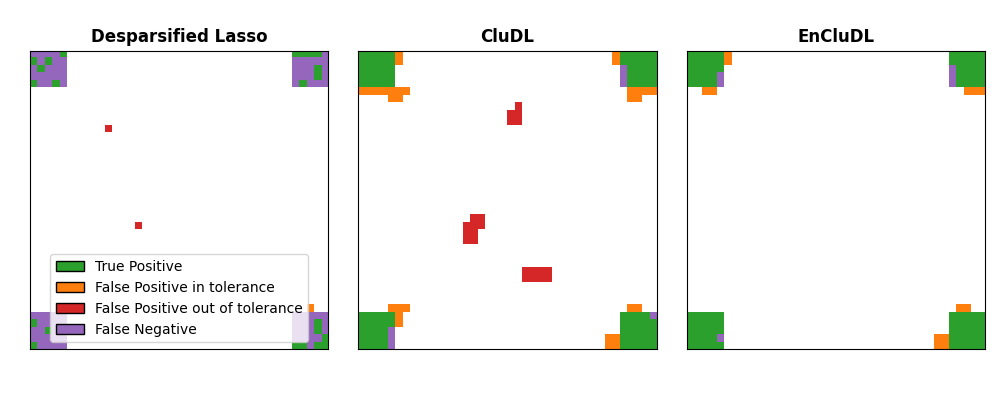
Comparison with spatial tolerance

Now, we compare the three methods presented above (Desparsified Lasso, CluDL and EnCluDL) in terms of support recovery with spatial tolerance.

def compute_spatially_relaxed_mask(mask, beta_extended):
    """Mark the false positives that are in the tolerance with a special value, -3"""
    support = beta_extended.reshape(shape) >= 1
    mask[support & (mask == -2)] = -3
    return mask


mask_dl_relaxed = compute_spatially_relaxed_mask(mask_dl, beta_extended)
mask_cludl_relaxed = compute_spatially_relaxed_mask(mask_cludl, beta_extended)
mask_encldl_relaxed = compute_spatially_relaxed_mask(mask_encludl, beta_extended)
cmap = ListedColormap(["tab:orange", "tab:red", "tab:purple", "white", "tab:green"])

# sphinx_gallery_thumbnail_number = 6
_, axes = plt.subplots(1, 3, figsize=(10, 4), subplot_kw={"xticks": [], "yticks": []})
axes[0].imshow(mask_dl_relaxed, cmap=cmap, vmin=-3, vmax=1)
axes[0].set_title("Desparsified Lasso", fontweight="bold")
axes[1].imshow(mask_cludl_relaxed, cmap=cmap, vmin=-3, vmax=1)
axes[1].set_title("CluDL", fontweight="bold")
axes[2].imshow(mask_encldl_relaxed, cmap=cmap, vmin=-3, vmax=1)
axes[2].set_title("EnCluDL", fontweight="bold")
legend_handles = [
    Patch(facecolor="tab:green", edgecolor="k", label="True Positive"),
    Patch(facecolor="tab:orange", edgecolor="k", label="False Positive in tolerance"),
    Patch(facecolor="tab:red", edgecolor="k", label="False Positive out of tolerance"),
    Patch(facecolor="tab:purple", edgecolor="k", label="False Negative"),
]
axes[0].legend(handles=legend_handles, loc="lower center")
plt.tight_layout()

Note: Choosing inference parameters

The choice of the number of clusters depends on several parameters, such as: the structure of the data (a higher correlation between neighboring features enable a greater dimension reduction, i.e. a smaller number of clusters), the number of samples (small datasets require more dimension reduction) and the required spatial tolerance (small clusters lead to limited spatial uncertainty). Formally, “spatial tolerance” is defined by the largest distance from the true support for which the occurrence of a false discovery is not statistically controlled (c.f. Chevalier et al.[4]). Theoretically, the spatial tolerance delta is equal to the largest cluster diameter. However this choice is conservative, notably in the case of ensembled clustered inference. For these algorithms, we recommend to take the average cluster radius. In this example, we choose n_clusters = 200, leading to a theoretical spatial tolerance delta = 6, which is still conservative (see Results).

References

[1]

Adel Javanmard and Andrea Montanari. Confidence intervals and hypothesis testing for high-dimensional regression. The Journal of Machine Learning Research, 15(1):2869–2909, 2014.

[2]

Cun-Hui Zhang and Stephanie S Zhang. Confidence intervals for low dimensional parameters in high dimensional linear models. Journal of the Royal Statistical Society Series B: Statistical Methodology, 76(1):217–242, 2014.

[3]

Sara van de Geer, Peter Bühlmann, Ya’acov Ritov, and Ruben Dezeure. On asymptotically optimal confidence regions and tests for high-dimensional models. The Annals of Statistics, pages 1166–1202, 2014.

[4] (1,2,3)

Jérôme-Alexis Chevalier, Tuan-Binh Nguyen, Bertrand Thirion, and Joseph Salmon. Spatially relaxed inference on high-dimensional linear models. Statistics and Computing, 32(5):83, 2022.

Estimated memory usage: 222 MB