Knockoff aggregation

The examples shows how to use aggregate model-X Knockoff selections to derandomize inference. The model-X Knockoff introduced by Candes et al.[1] allows for variable selection with statistical guarantees on the False Discovery Rate (FDR),

\[FDR = \mathbb{E}[ FDP ] = \mathbb{E} \left[ \frac{|\hat{S} \cap \mathcal{H}_0 | }{| \hat{S} |} \right]\]

where \(\hat{S}\) is the set of selected variables and \(\mathcal{H}_0\) is the set of null variables (i.e., variables with no effect on the response). A notable drawback of this procedure is the randomness associated with generating knockoff variables, \(\tilde{X}\). This can result in fluctuations of the statistical power and false discovery proportion, and consequently, unstable inference.

To mitigate this issue, several aggregation procedures have been proposed in the literature. Nguyen et al.[2] introduces a quantile aggregation procedure based on the p-values obtained from multiple independent runs of the knockoff filter. Or Ren and Barber[3] proposes an aggregation procedure based on e-values. We illustrate both procedures in this example.

Generating data

We use a simulated dataset where we know the ground truth to evaluate the performance, in terms of statistical power and false discovery proportion, of the different aggregation procedures. We generate data with n=300 samples and p=100 correlated features.

import numpy as np

from hidimstat._utils.scenario import multivariate_simulation

n_features = 100
n_samples = 300
# Correlation
rho = 0.5
# Sparsity of the support
sparsity = 0.5
# Signal-to-noise ratio
snr = 10

# Generate data
X, y, beta_true, noise = multivariate_simulation(
    n_samples=n_samples,
    n_features=n_features,
    rho=rho,
    support_size=int(n_features * sparsity),
    signal_noise_ratio=snr,
    seed=0,
)

Inference with model-X Knockoffs

We repeat the model-X Knockoff procedure multiple times, as controlled by the n_repeats parameter, to obtain different selections. This will allow us to observe the variability of the selections induced by the knockoff lottery. Then, we compare the possible solutions to aggregate the selections in order to derandomize the inference.

from hidimstat.knockoffs import ModelXKnockoff
from hidimstat.statistical_tools.multiple_testing import fdp_power

fdr = 0.1
n_repeats = 25
n_jobs = 4
model_x_knockoff = ModelXKnockoff(n_repeats=n_repeats, n_jobs=n_jobs, random_state=0)
model_x_knockoff.fit_importance(X, y)

fdp_individual = []
power_individual = []
model_x_knockoff.importances_.shape
for ko_statistics in model_x_knockoff.importances_:
    threshold = model_x_knockoff.knockoff_threshold(ko_statistics, fdr=fdr)
    ko_selection = ko_statistics > threshold

    fdp, power = fdp_power(ko_selection, ground_truth=beta_true)
    fdp_individual.append(fdp)
    power_individual.append(power)

/home/circleci/project/src/hidimstat/samplers/gaussian_knockoffs.py:205: UserWarning: The equi-correlated matrix for knockoffs is not positive definite. Reduce the value of distance by 2.220446049250313e-16.
  warnings.warn(
/home/circleci/project/src/hidimstat/samplers/gaussian_knockoffs.py:205: UserWarning: The equi-correlated matrix for knockoffs is not positive definite. Reduce the value of distance by 2.220446049250313e-15.
  warnings.warn(
/home/circleci/project/src/hidimstat/samplers/gaussian_knockoffs.py:205: UserWarning: The equi-correlated matrix for knockoffs is not positive definite. Reduce the value of distance by 2.220446049250313e-14.
  warnings.warn(

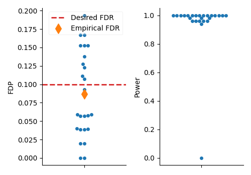
Visualize the results of the individual selections

We first visualize the results of the individual selections to observe the variability induced by the knockoff lottery. We plot the False Discovery Proportion (FDP) for each run along with the desired FDR level (red dashed line) and the statistical

import matplotlib.pyplot as plt
import pandas as pd
import seaborn as sns

df_plot = pd.DataFrame(
    {
        "FDP": fdp_individual,
        "Power": power_individual,
    }
)

_, axes = plt.subplots(1, 2, figsize=(5, 3.5))

ax = axes[0]
sns.swarmplot(
    data=df_plot,
    y="FDP",
    ax=ax,
)
ax.axhline(fdr, color="tab:red", linestyle="--", lw=2, label="Desired FDR")
ax.scatter(
    0,
    np.mean(fdp_individual),
    marker="d",
    color="tab:orange",
    s=100,
    zorder=10,
    label="Empirical FDR",
)
ax.legend(framealpha=0.2)
# Plot the power
ax = axes[1]
sns.swarmplot(
    data=df_plot,
    y="Power",
    ax=ax,
)
sns.despine()
_ = plt.tight_layout()

Aggregation procedures

We now compute the aggregation using both the p-values aggregation procedure from Nguyen et al.[2] and the e-values aggregation procedure from Ren and Barber[3]. We then compare the results of both procedures in terms of FDP and power.

pval_aggregation = model_x_knockoff.fdr_selection(fdr=fdr, adaptive_aggregation=True)
fdp_pval_agg, power_pval_agg = fdp_power(pval_aggregation, ground_truth=beta_true)

eval_aggregation = model_x_knockoff.fdr_selection(
    fdr=fdr, fdr_control="ebh", evalues=True
)
fdp_eval_agg, power_eval_agg = fdp_power(eval_aggregation, ground_truth=beta_true)

df_plot["Method"] = "Individual KO"
df_plot_2 = pd.concat(
    [
        df_plot,
        pd.DataFrame(
            {
                "FDP": [fdp_pval_agg],
                "Power": [power_pval_agg],
                "Method": ["P-value aggregation"],
            }
        ),
        pd.DataFrame(
            {
                "FDP": [fdp_eval_agg],
                "Power": [power_eval_agg],
                "Method": ["E-value aggregation"],
            }
        ),
    ],
    ignore_index=True,
)

# Plot the results
# ----------------
# In addition to the individual selections (blue), we plot the FDR and power obtained by
# p-value aggregation (orange) and e-value aggregation (green).

# sphinx_gallery_thumbnail_number = 2
_, axes = plt.subplots(1, 2, figsize=(6, 3.5))
ax = axes[0]
sns.stripplot(
    data=df_plot_2,
    y="FDP",
    hue="Method",
    ax=ax,
    palette="muted",
    dodge=1,
    legend=False,
    size=8,
    linewidth=1,
)
ax.axhline(fdr, color="tab:red", linestyle="--", lw=2, label="Desired FDR")

ax = axes[1]
sns.stripplot(
    data=df_plot_2,
    y="Power",
    hue="Method",
    ax=ax,
    palette="muted",
    dodge=True,
    size=8,
    linewidth=1,
)
sns.despine()
_ = plt.tight_layout()

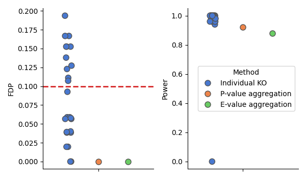
It appears that both aggregation procedures successfully lowers the false discovery proportion while maintaining a good statistical power.

References

[1]

Emmanuel Candes, Yingying Fan, Lucas Janson, and Jinchi Lv. Panning for gold:’model-x’ knockoffs for high dimensional controlled variable selection. Journal of the Royal Statistical Society Series B: Statistical Methodology, 80(3):551–577, 2018.

[2] (1,2)

Tuan-Binh Nguyen, Jerome-Alexis Chevalier, Bertrand Thirion, and Sylvain Arlot. Aggregation of multiple knockoffs. In Hal Daumé III and Aarti Singh, editors, Proceedings of the 37th International Conference on Machine Learning, volume 119 of Proceedings of Machine Learning Research, 7283–7293. PMLR, 2020.

[3] (1,2)

Zhimei Ren and Rina Foygel Barber. Derandomised knockoffs: leveraging e-values for false discovery rate control. Journal of the Royal Statistical Society Series B: Statistical Methodology, 86(1):122–154, 2023. doi:10.1093/jrsssb/qkad085.

Estimated memory usage: 215 MB