Conditional Randomization Test for Sparse Logistic Regression

This example demonstrates how to apply the distilled conditional randomization test (D0CRT) to logistic regression. The hidimstat package implements the decorrelation method described in Nguyen et al.[1], which ensures that the distribution of the test statistic under the null hypothesis closely approximates a standard Gaussian distribution. We illustrate this property by comparing the quantiles of the test statistics obtained using this method (dCRT-logit) with those from the original D0CRT.

Generate synthetic data for logistic regression

To begin, we’ll generate synthetic data for logistic regression. We’ll adapt the multivariate_simulation function to first create class probabilities using a logit link function, and then generate binary observations with a Bernoulli distribution. By simulating the data, we know the true underlying process and can identify which features are null. This information will be used to plot the quantiles of the test statistics under the null hypothesis.

import numpy as np
from scipy.special import expit

from hidimstat._utils.scenario import multivariate_simulation

# Simulation parameters
n_samples = 200
n_features = 100
support_size = 10
rho = 0.2  # strength of the serial correlation between adjacent features
signal_noise_ratio = 2.0

# Generate data for 5 different random seeds
X_list, y_list, beta_true_list = [], [], []
for seed in range(5):
    X, y_, beta_true, _ = multivariate_simulation(
        n_samples=n_samples,
        n_features=n_features,
        support_size=support_size,
        rho=rho,
        signal_noise_ratio=signal_noise_ratio,
        seed=seed,
    )
    X_list.append(X)
    # Transform y to binary using the logit link function
    y_logit = expit(y_)
    rng = np.random.default_rng(seed)
    y = rng.binomial(1, y_logit)
    y_list.append(y)
    beta_true_list.append(beta_true)

Compute the test statistics

Next, we compute the test statistics using both the dCRT and dCRT-logit methods. For dCRT-logit, we use a LogisticRegressionCV estimator; the D0CRT class automatically applies the decorrelation method. For dCRT, we use a LassoCV estimator, which implements the original Lasso-distillation approach described in Liu et al.[2]. We store the test statistic values for the null features only. The simulation uses n=200 samples and p=100 correlated features, with a support size of 10 and a signal-to-noise ratio of 3.0. The experiment is repeated for 5 different random seeds.

import pandas as pd
from sklearn.linear_model import LassoCV, LogisticRegressionCV

from hidimstat import D0CRT

# Run dCRT and dCRT-logit for each random seed
results_list = []
for seed, (X, y, beta_true) in enumerate(zip(X_list, y_list, beta_true_list)):

    # Fit the dCRT-logit model
    dcrt_logit = D0CRT(
        estimator=LogisticRegressionCV(
            penalty="l1",
            solver="liblinear",
            random_state=seed,
        ),
        screening_threshold=None,
        n_jobs=5,
    )
    dcrt_logit.fit(X, y)
    importance_logit = dcrt_logit.importance(X, y)
    power_logit = np.mean((dcrt_logit.pvalues_[beta_true] < 0.05))

    # Fit the dCRT with Lasso-distillation
    dcrt = D0CRT(
        estimator=LassoCV(random_state=seed, alphas=10, fit_intercept=False),
        screening_threshold=None,
        n_jobs=5,
    )
    dcrt.fit(X, y)
    importance = dcrt.importance(X, y)
    power = np.mean((dcrt.pvalues_[beta_true] < 0.05))

    # Store the results in a DataFrame
    results_list.append(
        pd.DataFrame(
            {
                "stat_dcrt": importance[~beta_true],
                "stat_dcrt_logit": importance_logit[~beta_true],
                "seed": seed,
                "power_dcrt": power,
                "power_dcrt_logit": power_logit,
            }
        )
    )


df_plot = pd.concat(results_list, ignore_index=True)

QQ-plot visualization

Next, we compare the quantiles of the test statistics from both methods to the theoretical quantiles of a standard Gaussian distribution. We use a QQ-plot, which displays the theoretical quantiles (from norm.ppf) against the empirical quantiles computed from the test statistics for each method.

import matplotlib.pyplot as plt
import seaborn as sns
from scipy.stats import norm

quantiles = np.linspace(1e-2, 1.0 - 1e-2, 100)
theoretical_quantiles = norm.ppf(quantiles)

empirical_quantiles = np.quantile(df_plot["stat_dcrt"], quantiles)
empirical_quantiles_logit = np.quantile(df_plot["stat_dcrt_logit"], quantiles)


_, axes = plt.subplots(1, 2, figsize=(6, 3), sharey=True, sharex=True)
sns.scatterplot(
    x=theoretical_quantiles,
    y=empirical_quantiles,
    ax=axes[0],
    edgecolor=None,
)
axes[0].plot(
    theoretical_quantiles, theoretical_quantiles, color="tab:red", ls="--", lw=2
)
axes[0].set_title("dCRT")
sns.scatterplot(
    x=theoretical_quantiles,
    y=empirical_quantiles_logit,
    ax=axes[1],
    edgecolor=None,
)
axes[1].plot(
    theoretical_quantiles, theoretical_quantiles, color="tab:red", ls="--", lw=2
)
axes[1].set_title("dCRT-logit")
axes[0].set_xlabel("Theoretical quantiles")
axes[0].set_ylabel("Empirical quantiles")
axes[1].set_xlabel("Theoretical quantiles")

sns.despine()
plt.tight_layout()

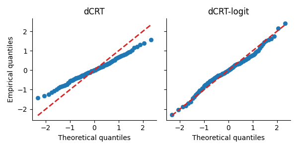
In the QQ-plot, the points for the dCRT-logit method are closer to the diagonal red dashed line compared to those for the dCRT method. This indicates that the test statistics from dCRT-logit more closely follow a standard Gaussian distribution under the null hypothesis.

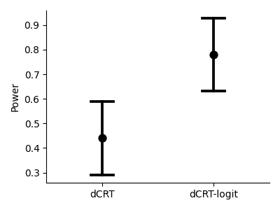
Power comparison

We also compare the statistical power of both methods. The plot below shows the average power across the 5 random seeds, with error bars representing the standard deviation.

_, ax = plt.subplots(figsize=(4, 3))
ax = sns.pointplot(
    data=df_plot[["power_dcrt", "power_dcrt_logit"]],
    errorbar="sd",
    capsize=0.2,
    linestyle="",
    c="k",
)
sns.despine()
ax.set_ylabel("Power")
ax.set_xticks([0, 1], labels=["dCRT", "dCRT-logit"])
plt.tight_layout()

References

[1]

Binh T Nguyen, Bertrand Thirion, and Sylvain Arlot. A conditional randomization test for sparse logistic regression in high-dimension. Advances in Neural Information Processing Systems, 35:13691–13703, 2022.

[2]

Molei Liu, Eugene Katsevich, Lucas Janson, and Aaditya Ramdas. Fast and powerful conditional randomization testing via distillation. Biometrika, 109(2):277–293, 2022.

Estimated memory usage: 215 MB