Pixel-wise inference on digit classification

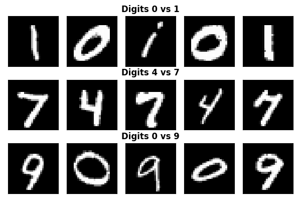
This example illustrates how to perform pixel-wise inference using Ensemble Clustered Inference with Desparsified Lasso (EnCluDL) on digit classification tasks. We use the MNIST dataset and consider binary classification between digits 1 vs 7 and 0 vs 1. The MNIST dataset contains 28x28 pixel images of handwritten digits.

Loading the MNIST dataset

We start by loading the MNIST dataset from OpenML. We then filter the dataset to include only digits 4 and 7 for the first classification task, and digits 0 and 1 for the second task and digits 0 and 9 for the third task. To speed up the example, we downsample the dataset to 4000 samples for each task.

import matplotlib.pyplot as plt
import numpy as np
from sklearn.datasets import fetch_openml
from sklearn.utils import resample

mnist_dataset = fetch_openml("mnist_784", version=1, as_frame=False)
X_mnist, y_mnist = mnist_dataset.data, mnist_dataset.target
# Downsample to speed up the example
n_samples = 5000
mask_4_7 = (y_mnist == "4") | (y_mnist == "7")
X_4_7, y_4_7 = X_mnist[mask_4_7], y_mnist[mask_4_7].astype(int)
X_4_7, y_4_7 = resample(
    X_4_7, y_4_7, n_samples=n_samples, replace=False, random_state=0, stratify=y_4_7
)

mask_0_1 = (y_mnist == "0") | (y_mnist == "1")
X_0_1, y_0_1 = X_mnist[mask_0_1], y_mnist[mask_0_1].astype(int)
X_0_1, y_0_1 = resample(
    X_0_1, y_0_1, n_samples=n_samples, replace=False, random_state=0, stratify=y_0_1
)

mask_0_9 = (y_mnist == "0") | (y_mnist == "9")
X_0_9, y_0_9 = X_mnist[mask_0_9], y_mnist[mask_0_9].astype(int)
X_0_9, y_0_9 = resample(
    X_0_9, y_0_9, n_samples=n_samples, replace=False, random_state=0, stratify=y_0_9
)

Visualizing samples from each classification task

_, axes = plt.subplots(3, 5, figsize=(6, 4), subplot_kw={"xticks": [], "yticks": []})
for i in range(5):
    # Plot 0 vs 1
    label = 1 if i % 2 == 0 else 0
    axes[0, i].imshow(X_0_1[y_0_1 == label][i].reshape(28, 28), cmap="gray")
    # Plot 4 vs 7
    label = 7 if i % 2 == 0 else 4
    axes[1, i].imshow(X_4_7[y_4_7 == label][i].reshape(28, 28), cmap="gray")
    # PLot 0 vs 9
    label = 9 if i % 2 == 0 else 0
    axes[2, i].imshow(X_0_9[y_0_9 == label][i].reshape(28, 28), cmap="gray")

axes[0, 2].set_title("Digits 0 vs 1", fontweight="bold", y=1.0)
axes[1, 2].set_title("Digits 4 vs 7", fontweight="bold", y=1.0)
axes[2, 2].set_title("Digits 0 vs 9", fontweight="bold", y=1.0)

_ = plt.tight_layout()

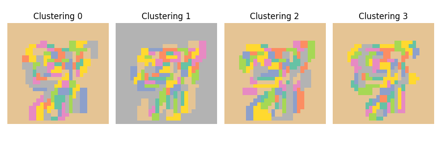
Randomness in clustering affects inference stability

A key limitation of clustered inference procedures is that the clustering step introduces randomness into the inference process. Data perturbations can produce different clustering results, which subsequently lead to varying inference outcomes. This effect can be demonstrated by running the clustering algorithm multiple times on different subsamples of the data. Here we use the Ward hierarchical clustering algorithm with spatial connectivity constraints (each pixel is connected to its immediate neighbors) to cluster the pixels of the images. We use 100 clusters and visualize the clustering results for four different subsamples of the data.

from sklearn.cluster import FeatureAgglomeration
from sklearn.feature_extraction import image

n_clusters = 100
shape = (28, 28)
connectivity = image.grid_to_graph(n_x=shape[0], n_y=shape[1])


_, axes = plt.subplots(1, 4, figsize=(9, 3))

for i, ax in enumerate(axes):
    X_cluster = resample(X_4_7, n_samples=n_samples // 2, replace=False, random_state=i)
    clustering = FeatureAgglomeration(n_clusters=n_clusters, connectivity=connectivity)
    clustering.fit(X_cluster)
    ax.imshow(clustering.labels_.reshape(28, 28), cmap="Set2")
    ax.axis("off")
    ax.set_title(f"Clustering {i}")

_ = plt.tight_layout()

Ensemble Clustered Inference with Desparsified Lasso

To mitigate the randomness introduced by clustering, we ensemble the results from multiple clustered inference procedures. This approach derandomizes the inference procedure and produces more stable results. We use the class:hidimstat.EnCluDL for this purpose with 10 bootstraps. While this approach is more computationally intensive than single clustered inference, the procedure can be parallelized across clustering repetitions using the n_jobs parameter.

from sklearn.cluster import FeatureAgglomeration
from sklearn.feature_extraction import image
from sklearn.linear_model import LassoCV

from hidimstat import DesparsifiedLasso
from hidimstat.ensemble_clustered_inference import EnCluDL

fwer = 0.1
n_jobs = 5
n_clusters = 100

encludl = EnCluDL(
    clustering=clustering,
    desparsified_lasso=DesparsifiedLasso(estimator=LassoCV(max_iter=1000)),
    n_bootstraps=10,
    n_jobs=n_jobs,
    random_state=0,
    cluster_boostrap_size=0.5,
)

encludl.fit_importance(X_4_7, y_4_7)
selected_4_7 = encludl.fwer_selection(
    fwer=fwer, n_tests=n_clusters, two_tailed_test=True
)

encludl.fit_importance(X_0_1, y_0_1)
selected_0_1 = encludl.fwer_selection(
    fwer=fwer, n_tests=n_clusters, two_tailed_test=True
)

encludl.fit_importance(X_0_9, y_0_9)
selected_0_9 = encludl.fwer_selection(
    fwer=fwer, n_tests=n_clusters, two_tailed_test=True
)

Fitting clustered inferences:   0%|          | 0/10 [00:00<?, ?it/s]
Fitting clustered inferences: 100%|██████████| 10/10 [00:01<00:00,  6.38it/s]
Fitting clustered inferences: 100%|██████████| 10/10 [00:01<00:00,  6.37it/s]

Computing importances:   0%|          | 0/10 [00:00<?, ?it/s]
Computing importances: 100%|██████████| 10/10 [00:00<00:00, 555.02it/s]

Fitting clustered inferences:   0%|          | 0/10 [00:00<?, ?it/s]
Fitting clustered inferences: 100%|██████████| 10/10 [00:02<00:00,  4.09it/s]
Fitting clustered inferences: 100%|██████████| 10/10 [00:02<00:00,  4.09it/s]

Computing importances:   0%|          | 0/10 [00:00<?, ?it/s]
Computing importances: 100%|██████████| 10/10 [00:00<00:00, 387.02it/s]

Fitting clustered inferences:   0%|          | 0/10 [00:00<?, ?it/s]
Fitting clustered inferences: 100%|██████████| 10/10 [00:02<00:00,  4.43it/s]
Fitting clustered inferences: 100%|██████████| 10/10 [00:02<00:00,  4.43it/s]

Computing importances:   0%|          | 0/10 [00:00<?, ?it/s]
Computing importances: 100%|██████████| 10/10 [00:00<00:00, 664.62it/s]

Visualizing the results

Finally, we visualize the significant pixels identified by EnCluDL for each of the three classification tasks.

import matplotlib.pyplot as plt
from matplotlib.colors import ListedColormap

_, axes = plt.subplots(1, 3, figsize=(5, 2), subplot_kw={"xticks": [], "yticks": []})

for i, (title, selected) in enumerate(
    [
        ("4 vs 7", selected_4_7),
        ("0 vs 1", selected_0_1),
        ("0 vs 9", selected_0_9),
    ]
):
    mask_encludl = selected.reshape(shape)

    cmap = ListedColormap(["tab:red", "white", "tab:blue"])
    axes[i].imshow(mask_encludl, cmap=cmap, vmin=-1, vmax=1)
    axes[i].set_title(title, fontweight="bold", y=1.0)

plt.tight_layout()

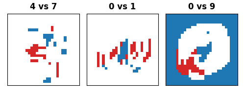
Performing inference on handwritten digits is challenging because the images are not perfectly aligned, and the pixel regions occupied by digits vary from one image to another. However, using EnCluDL, we can still identify clusters of pixels that are statistically significant for the classification tasks. For example, we can detect the bottom left portion of the loop when distinguishing between digits 0 and 9, the bottom left corner of digit 4 when distinguishing between digits 4 and 7, and the central vertical stroke when distinguishing between digits 0 and 1.

Estimated memory usage: 1442 MB