Leave-One-Covariate-In (LOCI) feature importance with different regression models

This example demonstrates how to compare LOCI feature importance [Williamson et al.[1]] across different predictive models on the same regression dataset. LOCI is model-agnostic and can be applied to any predictive model. Here, we use a linear model, a random forest, a neural network, and a support vector machine. We compare the models based on their predictive performance (R2 score) and the LOCI feature importance they yield.

Loading and preparing the data

We begin by simulating a regression dataset with 10 features, 5 of which are in the support set, meaning they contribute to generating the outcome. In this example, we use a simulated dataset to have access to the true support set of features and evaluate how well the different models identify these important features. The data is then split into training and test sets. These sets are used both to fit the predictive models and within the LOCI procedure, which refits models on subsets of features that exclude the feature of interest.

from sklearn.datasets import make_regression
from sklearn.model_selection import train_test_split

X, y, beta = make_regression(
    n_samples=300,
    n_features=10,
    n_informative=5,
    random_state=0,
    coef=True,
    noise=4.0,
)

# We convert the coefficients of the data-generating process into a binary array
# indicating the true support set of features.
beta = beta != 0

X_train, X_test, y_train, y_test = train_test_split(
    X,
    y,
    test_size=0.2,
    random_state=0,
    shuffle=True,
)

Fitting models and computing LOCI feature importance

We define a list of predictive models to compare. We use RidgeCV for linear regression, RandomForestRegressor for a tree-based model, MLPRegressor for a neural network, and SVR for a support vector machine, with RBF kernel. We then fit each model on the training data, compute the LOCI feature importance on the test data, and store the results in a DataFrame for comparison. Beware on the choice of hyperparameters of certain models to avoid over-fitting.

import pandas as pd
from sklearn.ensemble import RandomForestRegressor
from sklearn.linear_model import RidgeCV
from sklearn.metrics import mean_squared_error
from sklearn.neural_network import MLPRegressor
from sklearn.svm import SVR

from hidimstat import LOCI

models_list = [
    RidgeCV(),
    MLPRegressor(
        hidden_layer_sizes=(8),
        random_state=0,
        max_iter=500,
        learning_rate_init=0.1,
    ),
    SVR(kernel="linear"),
    RandomForestRegressor(
        n_estimators=50, max_depth=3, min_samples_leaf=10, random_state=0
    ),
]

df_list = []
for model in models_list:
    # Fit the full model
    model = model.fit(X_train, y_train)
    loci = LOCI(model, method="predict", loss=mean_squared_error)
    # Refit the model on a single feature / group of feature, and compute LOCI
    # importance. This process is repeated for all features / groups of features to assess
    # their individual contributions.
    loci.fit(X_train, y_train)
    importances = loci.importance(X_test, y_test)
    df_list.append(
        pd.DataFrame(
            {
                "feature": list(range(X.shape[1])),
                "importance": importances,
                "model": model.__class__.__name__,
                "R2 score": model.score(X_test, y_test),
            }
        )
    )

The predictive performance of the models can be compared using their R2 scores. This helps assess how effectively each model captures the underlying data-generating process.

df_plot = pd.concat(df_list)
df_plot.groupby("model").mean()["R2 score"].to_frame()

	R2 score
model
MLPRegressor	0.998202
RandomForestRegressor	0.632126
RidgeCV	0.999342
SVR	0.997806

Visualization of LOCI feature importance

Finally, we visualize the LOCI feature importance for each model using a horizontal bar plot. The true support features are highlighted in the plot with a green shaded background.

import matplotlib.pyplot as plt
import seaborn as sns

ax = sns.barplot(
    data=df_plot,
    y="feature",
    x="importance",
    hue="model",
    palette="muted",
    orient="h",
)
sns.despine()

for i, support in enumerate(beta):
    if support != 0:
        ax.axhspan(
            i - 0.45,
            i + 0.45,
            color="tab:olive",
            alpha=0.3,
            zorder=-1,
            label="True Support" if i == 1 else None,
        )
ax.legend()
plt.show()

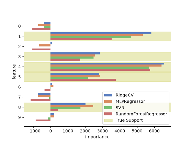
The plot shows that the different models all identify the true support features and assign them higher importance scores. However, the magnitude of the importance scores varies across models. It can be observed that models with a greater predictive performance (higher R2 score) tend to assign higher importance scores to the true support features.

Conclusion

LOCI is a simple and easily-interpretable method that can be used in parallel to LOCO to obtain a different interpretation of variable importance. Please keep in mind that models are fit on single features, which can lead to overfitting depending on the hyperparameters. One way to counteract this is to use LOCICV which can reduce noise for high-variance or unregularized models.

References

[1]

Brian D. Williamson, Peter B. Gilbert, Noah R. Simon, and Marco Carone. A General Framework for Inference on Algorithm-Agnostic Variable Importance. Journal of the American Statistical Association, 118(543):1645–1658, 2023. doi:10.1080/01621459.2021.2003200.

Estimated memory usage: 220 MB