Conditional vs Marginal Importance on the XOR dataset

This example illustrates on XOR data that variables can be conditionally important even if they are not marginally important. The conditional importance is computed using the Conditional Permutation Importance (CPI) class and the marginal importance is computed using univariate models.

import matplotlib.pyplot as plt
import numpy as np
import seaborn as sns
from sklearn.base import clone
from sklearn.linear_model import RidgeCV
from sklearn.metrics import hinge_loss
from sklearn.model_selection import KFold, train_test_split
from sklearn.svm import SVC

from hidimstat import CPI

To solve the XOR problem, we will use a Support Vector Classier (SVC) with Radial Basis Function (RBF) kernel. The decision function of the fitted model shows that the model is able to separate the two classes.

rng = np.random.RandomState(0)
X = rng.randn(400, 2)
Y = np.logical_xor(X[:, 0] > 0, X[:, 1] > 0).astype(int)

xx, yy = np.meshgrid(
    np.linspace(np.min(X[:, 0]), np.max(X[:, 0]), 100),
    np.linspace(np.min(X[:, 1]), np.max(X[:, 1]), 100),
)

X_train, X_test, y_train, y_test = train_test_split(X, Y, test_size=0.2, random_state=0)
model = SVC(kernel="rbf", random_state=0)
model.fit(X_train, y_train)
Z = model.decision_function(np.c_[xx.ravel(), yy.ravel()])

Visualizing the decision function of the SVC

fig, ax = plt.subplots()
ax.imshow(
    Z.reshape(xx.shape),
    interpolation="nearest",
    extent=(xx.min(), xx.max(), yy.min(), yy.max()),
    cmap="RdYlBu_r",
    alpha=0.6,
    origin="lower",
    aspect="auto",
)
sns.scatterplot(
    x=X[:, 0],
    y=X[:, 1],
    hue=Y,
    ax=ax,
    palette="muted",
)
ax.axis("off")
ax.legend(
    title="Class",
)
ax.set_title("Decision function of SVC with RBF kernel")
plt.show()

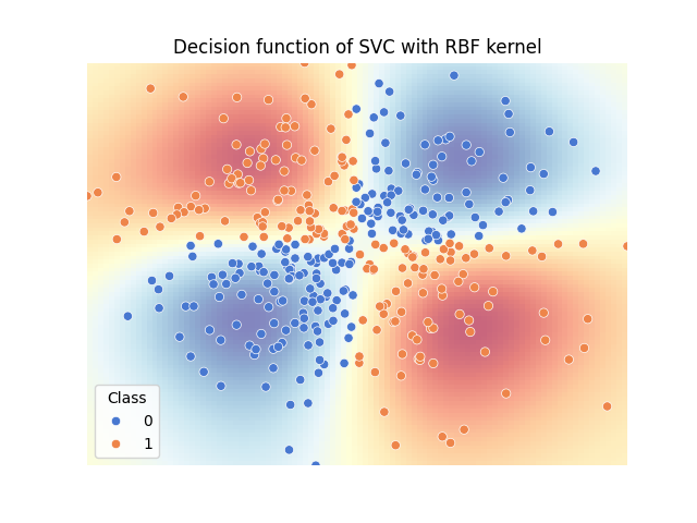
The decision function of the SVC shows that the model is able to learn the non-linear decision boundary of the XOR problem. It also highlights that knowing the value of both features is necessary to classify each sample correctly.

Computing the conditional and marginal importance

We first compute the marginal importance by fitting univariate models on each feature. Then, we compute the conditional importance using the CPI class. The univarariate models don’t perform above chance, since solving the XOR problem requires to use both features. Conditional importance, on the other hand, reveals that both features are important (therefore rejecting the null hypothesis \(Y \perp\!\!\!\perp X^1 | X^2\)).

cv = KFold(n_splits=5, shuffle=True, random_state=0)
clf = SVC(kernel="rbf", random_state=0)
# Compute marginal importance using univariate models
marginal_scores = []
for i in range(X.shape[1]):
    feat_scores = []
    for train_index, test_index in cv.split(X):
        X_train, X_test = X[train_index], X[test_index]
        y_train, y_test = Y[train_index], Y[test_index]

        X_train_univariate = X_train[:, i].reshape(-1, 1)
        X_test_univariate = X_test[:, i].reshape(-1, 1)

        univariate_model = clone(clf)
        univariate_model.fit(X_train_univariate, y_train)

        feat_scores.append(univariate_model.score(X_test_univariate, y_test))
    marginal_scores.append(feat_scores)

importances = []
for i, (train_index, test_index) in enumerate(cv.split(X)):
    X_train, X_test = X[train_index], X[test_index]
    y_train, y_test = Y[train_index], Y[test_index]

    clf_c = clone(clf)
    clf_c.fit(X_train, y_train)

    vim = CPI(
        estimator=clf_c,
        method="decision_function",
        loss=hinge_loss,
        imputation_model_continuous=RidgeCV(np.logspace(-3, 3, 10)),
        n_permutations=50,
        random_state=0,
    )
    vim.fit(X_train, y_train)
    importances.append(vim.importance(X_test, y_test)["importance"])

importances = np.array(importances).T

Visualizing the importance scores

We will use boxplots to visualize the distribution of the importance scores.

fig, axes = plt.subplots(1, 2, sharey=True, figsize=(6, 2.5))
# Marginal scores boxplot
sns.boxplot(
    data=np.array(marginal_scores).T,
    orient="h",
    ax=axes[0],
    fill=False,
    color="C0",
    linewidth=3,
)
axes[0].axvline(x=0.5, color="k", linestyle="--", lw=3)
axes[0].set_ylabel("")
axes[0].set_yticks([0, 1], ["X1", "X2"])
axes[0].set_xlabel("Marginal Scores (accuracy)")
axes[0].set_ylabel("Features")

# Importances boxplot
sns.boxplot(
    data=np.array(importances).T,
    orient="h",
    ax=axes[1],
    fill=False,
    color="C0",
    linewidth=3,
)
axes[1].set_xlabel("Conditional Importance")
axes[1].axvline(x=0.0, color="k", linestyle="--", lw=3)
plt.tight_layout()
plt.show()

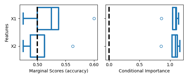
On the left, we can see that both features are not marginally important, since the boxplots overlap with the chance level (accuracy = 0.5). On the right, we can see that both features are conditionally important, since the importance scores are far from the null hypothesis (importance = 0.0).