Note
Go to the end to download the full example code.
Controlled multiple variable selection on the Wisconsin breast cancer dataset#
In this example, we explore the basics of variable selection and illustrate the need to statistically control the amount of faslely selected variables. We compare two variable selection methods: the Lasso and the Model-X Knockoffs Candes et al.[1]. We show how the Lasso is not robust to the presence of irrelevant variables, while the Knockoffs (KO) method is able to address this issue.
import numpy as np
import pandas as pd

seed = 0
rng = np.random.RandomState(seed)
Load the breast cancer dataset#
There are 569 samples and 30 features that correspond to tumor attributes. The downstream task is to classify tumors as benign or malignant. We leave out 10% of the data to evaluate the performance of the Logistic Lasso (Logistic Regression with L1 regularization) on the prediction task.
from sklearn.datasets import load_breast_cancer
from sklearn.model_selection import train_test_split
from sklearn.preprocessing import StandardScaler

data = load_breast_cancer()
X = data.data
y = data.target

X_train, X_test, y_train, y_test = train_test_split(
    X, y, test_size=0.1, random_state=seed
)

scaler = StandardScaler()
X_train = scaler.fit_transform(X_train)
X_test = scaler.transform(X_test)
n_train, p = X_train.shape
n_test = X_test.shape[0]
feature_names = [str(name) for name in data.feature_names]
Selecting variables with the Logistic Lasso#
We want to select variables that are relevant to the outcome, i.e. tumor charateristics that are associated with tumor malignance. We start off by applying a classical method using Lasso logistic regression and retaining variables with non-null coefficients:
from sklearn.linear_model import LogisticRegressionCV

clf = LogisticRegressionCV(
    Cs=np.logspace(-3, 3, 10), penalty="l1", solver="liblinear", random_state=rng
)
clf.fit(X_train, y_train)
print(f"Accuracy of Lasso on test set: {clf.score(X_test, y_test):.3f}")


selected_lasso = np.where(np.abs(clf.coef_[0]) > 1e-6)[0]
print(f"The Lasso selects {len(selected_lasso)} variables:")
print(f"{'Variable name':<30} | {'Coefficient':>10}")
print("-" * 45)
for i in selected_lasso:
    print(f"{feature_names[i]:<30} | {clf.coef_[0][i]:>10.3f}")
Accuracy of Lasso on test set: 1.000
The Lasso selects 8 variables:
Variable name                  | Coefficient
---------------------------------------------
mean concave points            |     -0.438
radius error                   |     -0.572
worst radius                   |     -2.274
worst texture                  |     -0.603
worst smoothness               |     -0.223
worst concavity                |     -0.062
worst concave points           |     -0.939
worst symmetry                 |     -0.147
Evaluating the rejection set#
Since we do not have the ground truth for the selected variables (i.e. we do not know the relationship between the tumor characteristics and the the malignance of the tumor ), we cannot evaluate this selection set directly. To investigate the reliability of this method, we artificially increase the number of variables by adding noisy copies of the features. These are correlated with the variables in the dataset, but are not related to the outcome.
repeats_noise = 5  # Number of synthetic noisy sets to add

noises_train = [X_train]
noises_test = [X_test]
feature_names_noise = [x for x in feature_names]
for k in range(repeats_noise):
    X_train_c = X_train.copy()
    X_test_c = X_test.copy()
    noises_train.append(X_train_c + 2 * rng.randn(n_train, p))
    noises_test.append(X_test_c + 2 * rng.randn(n_test, p))
    feature_names_noise += [f"spurious #{k*p+i}" for i in range(p)]

noisy_train = np.concatenate(noises_train, axis=1)
noisy_test = np.concatenate(noises_test, axis=1)
There are 180 features, 30 of them are real and 150 of them are fake and independent of the outcome. We now apply the Lasso (with cross-validation to select the best regularization parameter) to the noisy dataset and observe the results:
lasso_noisy = LogisticRegressionCV(
    Cs=np.logspace(-3, 3, 10),
    penalty="l1",
    solver="liblinear",
    random_state=rng,
    n_jobs=1,
)
lasso_noisy.fit(noisy_train, y_train)
y_pred_noisy = lasso_noisy.predict(noisy_test)
print(
    f"Accuracy of Lasso on test set with noise: {lasso_noisy.score(noisy_test, y_test):.3f}"
)

selected_mask = [
    "selected" if np.abs(x) > 1e-6 else "not selected" for x in lasso_noisy.coef_[0]
]
df_lasso_noisy = pd.DataFrame(
    {
        "score": np.abs(lasso_noisy.coef_[0]),
        "variable": feature_names_noise,
        "selected": selected_mask,
    }
)
# Count how many selected features are actually noise
num_false_discoveries = np.sum(
    np.array(selected_mask[p:]) == "selected"
)  # Count the number of selected spurious variables
print(f"The Lasso makes at least {num_false_discoveries} False Discoveries!!")
Accuracy of Lasso on test set with noise: 0.947
The Lasso makes at least 109 False Discoveries!!
The Lasso selects many spurious variables that are not directly related to the outcome. To mitigate this problem, we can use one of the statistically controlled variable selection methods implemented in hidimstat. This ensures that the proportion of False Discoveries is below a certain bound set by the user in all scenarios.
Controlled variable selection with Knockoffs#
We use the Model-X Knockoff procedure to control the FDR (False Discovery Rate). The selection of variables is based on the Lasso Coefficient Difference (LCD) statistic Candes et al.[1].
from hidimstat import model_x_knockoff

fdr = 0.2

selected, test_scores, threshold, X_tildes = model_x_knockoff(
    noisy_train,
    y_train,
    estimator=LogisticRegressionCV(
        solver="liblinear",
        penalty="l1",
        Cs=np.logspace(-3, 3, 10),
        random_state=rng,
        tol=1e-3,
        max_iter=1000,
    ),
    n_bootstraps=1,
    random_state=0,
    tol_gauss=1e-15,
    preconfigure_estimator=None,
    fdr=fdr,
)

# Count how many selected features are actually noise
num_false_discoveries = np.sum(selected >= p)
print(f"Knockoffs make at least {num_false_discoveries} False Discoveries")
Knockoffs make at least 0 False Discoveries
Visualizing the results#
We can compare the selection sets obtained by the two methods. In addition to the binary selection (selected or not), we can also visualize the the KO statistic along with the selection threshold for the knockoffs and the absolute value of the Lasso coefficients. We plot the 25 most important features according to the KO statistic.
import matplotlib.pyplot as plt
import seaborn as sns

selected_mask = np.array(["not selected"] * len(test_scores))
selected_mask[selected] = "selected"
df_ko = pd.DataFrame(
    {
        "score": test_scores,
        "variable": feature_names_noise,
        "selected": selected_mask,
    }
)
df_ko = df_ko.sort_values(by="score", ascending=False).head(25)

fig, axes = plt.subplots(
    1,
    2,
    sharey=True,
)
ax = axes[0]
sns.scatterplot(
    data=df_ko,
    x="score",
    y="variable",
    hue="selected",
    ax=ax,
    palette={"selected": "tab:red", "not selected": "tab:gray"},
)
ax.axvline(x=threshold, color="k", linestyle="--", label="Threshold")
ax.legend()
ax.set_xlabel("KO statistic (LCD)")
ax.set_ylabel("")
ax.set_title("Knockoffs", fontweight="bold")

ax = axes[1]
sns.scatterplot(
    data=df_lasso_noisy[df_lasso_noisy["variable"].isin(df_ko["variable"])],
    x="score",
    y="variable",
    hue="selected",
    ax=ax,
    palette={"selected": "tab:red", "not selected": "tab:gray"},
    legend=False,
)
ax.set_xlabel("$|\\hat{\\beta}|$")
ax.axvline(
    x=0,
    color="k",
    linestyle="--",
)
ax.set_title("Lasso", fontweight="bold")
plt.tight_layout()
plt.show()
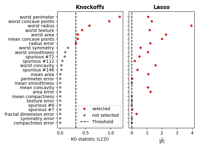
We can clearly see that the knockoffs procedure is more conservative than the Lasso and rejects the spurious features while many of them are selected by the Lasso. It is also interesting to note that some of the selected variables (with the high KO statistic (e.g., worst radius, worst area, mean concave points) are also variables with the largest Lasso coefficients.
References#
Total running time of the script: (0 minutes 8.341 seconds)